
No one can escape math. As a small business owner, you will be an accountant, office cleaner, employee and a I.T. support tech. If there is a function in the business that needs doing, you will have probably tried doing it. As an accountant, you will need some essential spreadsheet formulas for small business.
These formulas work in Apache Open Office Calc, Microsoft Excel, Apple Numbers and Google Sheets
SUMIF
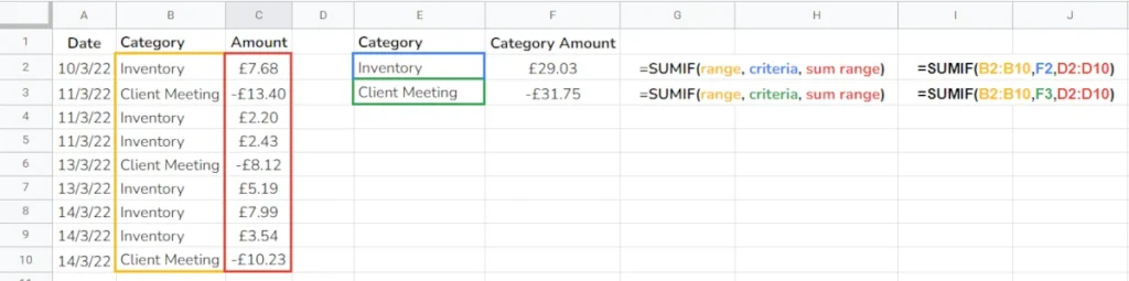
SUMIF is great for expense tracking and analysis. Being able to see what categories of products are selling or where expenses are getting out of hand is key to running any business. SUMIF looks at a range for criteria and adds every one that meets that criteria.
=SUMIF(range, criteria, sum range)
=SUMIF(B2:B10,F2,D2:D10)
AVERAGE
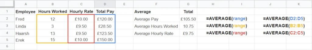
Do you need to know the average cost of products or the average hourly rate of employees? We have a spreadsheet formula to help. It’s surprising how useful knowing what an average is. One low or high figure, like Linda in the below example can heavily affect averages.
=AVERAGE(range)
=AVERAGE(B2:B5)
COUNTIF
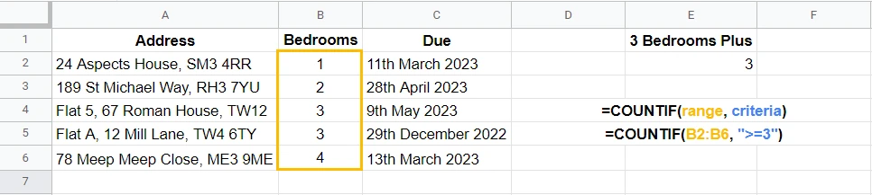
Only yesterday we received a spreadsheet by a client with details of a potential contract. I wanted to know how many properties required job X and how many required job Y. To easily work this out; we used COUNTIF. This formula will count how many items in a list that meet specific criteria. For us, we had a list of addresses, amount of bedrooms, and dates due. We just wanted to know how many of these properties had 3 or more bedrooms.
=COUNTIF(range, criteria)
=COUNTIF(B2:B6, “>=3”)
TRIM
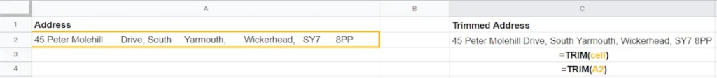
If we have a set of bad quality data, we may fix it with TRIM. This formula will remove unnecessary spaces from a cell and display easy-to-read data. TRIM will only work on a single cell and not a range, giving it the downside of a spreadsheet appearing to have duplicate data. But you can use TRIM, copy the new column or row and use Paste Values.
=TRIM(cell)
=TRIM(A2)
Conditional formatting
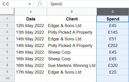
Essential spreadsheet formulas last entry is conditional formatting is a method of applying colour, style, font size, etc based on a specific cell contents. The best example of this is our bank balance -£97 when a figure is under £0, they display it in red. We can use conditional formatting to highlight specific words, numbers over a threshold, numbers smaller than 10% of 67 and anything else you can think of. Conditional formatting uses basic and advanced spreadsheet formulas.

How to use conditional formatting
Equipment
- Spreadsheet Software
Ingredients
- Spreadsheet
- Spreadsheet
Instructions
Google Sheets and Apache Open Office Calc
- Select the Row, Column or group of cells you wish to apply the formatting to
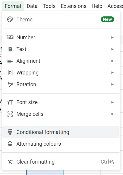
- Format > Conditional formatting in the top menu
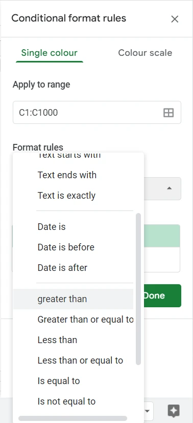
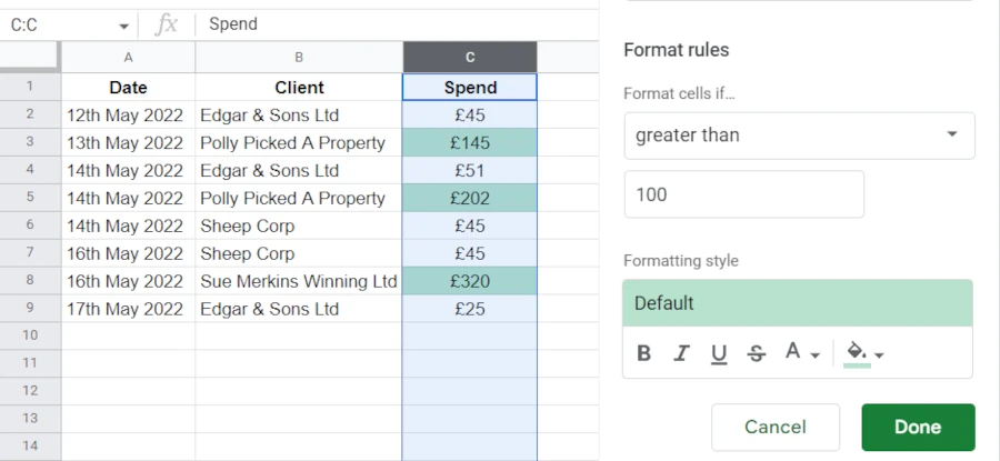
- Apply to range will be auto completed with your original selectionWe now can set Format rules, from the drop down select a rule you with to useWe will be using Greater than
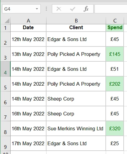
- Under the drop down we can add what number the cell should be greater thanWe have used 100, you can see the column change as soon as you input a number
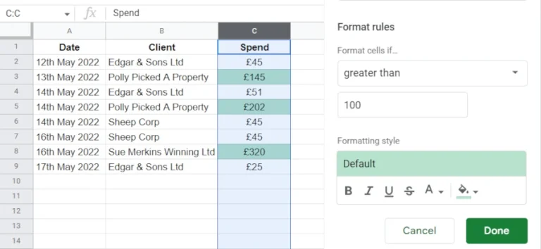
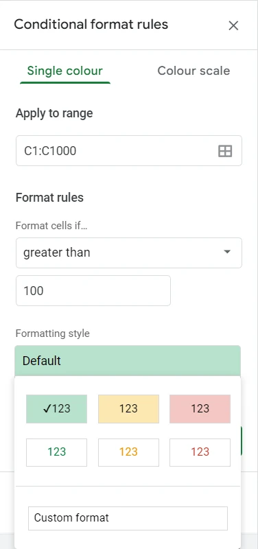
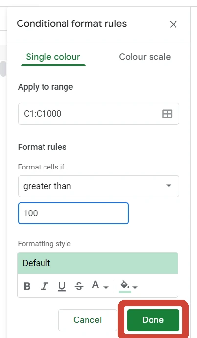
- Next we can change the Formatting style. Use one of the predefined styles or create your own Custom style
- Once happy press OK
Microsoft Excel
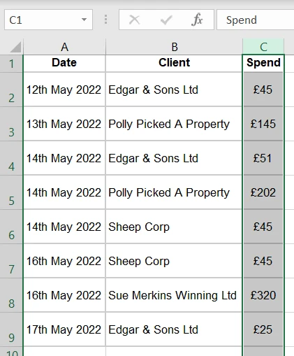
- Select the Row, Column or group of cells you wish to apply the formatting to
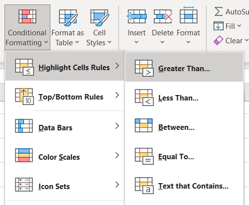
- Home > Conditional Formatting (In the styles section)Use the drop-down menu to select the type of rule you want to apply. You can use rules like greater than, less than, contains text, is exactly, etc.
- On the left set your requirements, In our example we want all £100+ highlightedOn the right we have the choose of some basic styles
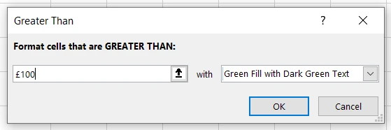
- Once happy press OK
Struggling with the above recipe? Hire a chef to do it for you